
Extra: Variable mechanical advantage in series-elastic actuators
Finding the best way to accelerate a mass using a motor and spring


We want the robot squirrel to be able to propel itself very far (continuously), but the motor is only so powerful, and the leg only so long. What strategies can be used to guide our leg design goals so the squirrel jumps higher than existing designs?
This post records my exploration of varying the mechanical advantage in a series-elastic actuator so that it moves an object as fast as possible, within a given time and distance. I’ll first review some ideas from literature and intuition, then show the process of generating the optimal strategy given a model of the system. I hope to explain things for a broader audience, so let me know if anything is confusing!
Human thoughts
Energy is power multiplied by time, so to get more kinetic energy out of the same motor, we can:
Increase power output by getting the motor to operate closer to its maximum power point
Increase the time that the power is applied by getting the motor to run for longer
More power
DC electric motors output the most power at the middle of their operating point. The relationship between torque and speed is roughly linear, so it’s strongest when it’s not spinning, and spins the fastest when there is no load. At the halfway point, the power (calculated by torque * speed) is at a maximum.

Direct Drive
One way to keep the motor operating at the maximum power point is to vary the mechanical advantage of the system, defined by the ratio of speed in/speed out, also equivalent to force out/force in. When a bicyclist shifts gears to go faster, they change the gear ratio so their legs can keep moving at the same speed but the wheel spins faster. Similarly, a jumping robot leg mechanism should decrease the mechanical advantage as the leg extends so the motor at the input can stay at its best speed.
Minitaur by Ghost Robotics is direct-drive1, meaning there is no gear reduction between the motor and the leg. However, it uses a clever linkage that decreases the mechanical advantage for the initial part of the extension when the “knee” joints move down, making the leg move faster for the same motor rotation speed.
Series-elasticity
Another way to keep a motor near its maximum power point is with a series elastic actuator2:

Putting a spring in between the motor and the leg means that any position differences between the motor and the leg store energy. If the leg starts from rest, for the first bit of movement the motor can spin quite fast as it winds up the spring. As the spring deforms more, the leg feels more force and starts to move. At some point, the leg can move even faster than the geared output of the motor because the stored energy in the spring is released.
In the left plot below, if the spring is really stiff (acting like a rigid joint between the red and blue masses), the motor starts slow and keeps increasing. The torque keeps decreasing, and the power only reaches the peak for a moment. With the less stiff spring on the right, the motor speeds up quickly and spends more time around the middle of its operating range. By balancing speed and torque better, the average power over the entire time period is higher.

More time
The other way to increase energy output is to allow for more time to build up energy. When I flick something, I store elastic energy in my tendons and then suddenly release it to get more instantaneous power at my finger than otherwise possible.
Similarly, the series-elastic robot leg can store a lot more energy by holding the leg still at the output, winding up spring through the motor, then suddenly releasing the leg. Another benefit of storing energy by holding the leg is that it allows for shorter legs to work just as well as longer ones. With direct-drive legs where the leg is always in the process of extending, there is an upper limit for the amount of time that power can be applied. With energy storage, leg length is less of a restriction.
One way to look at it is that we want to maximize the ending velocity of the mass being accelerated. However, there is only a certain allowable change in position (the max leg length), which can be represented by the area under the velocity vs. time curve:
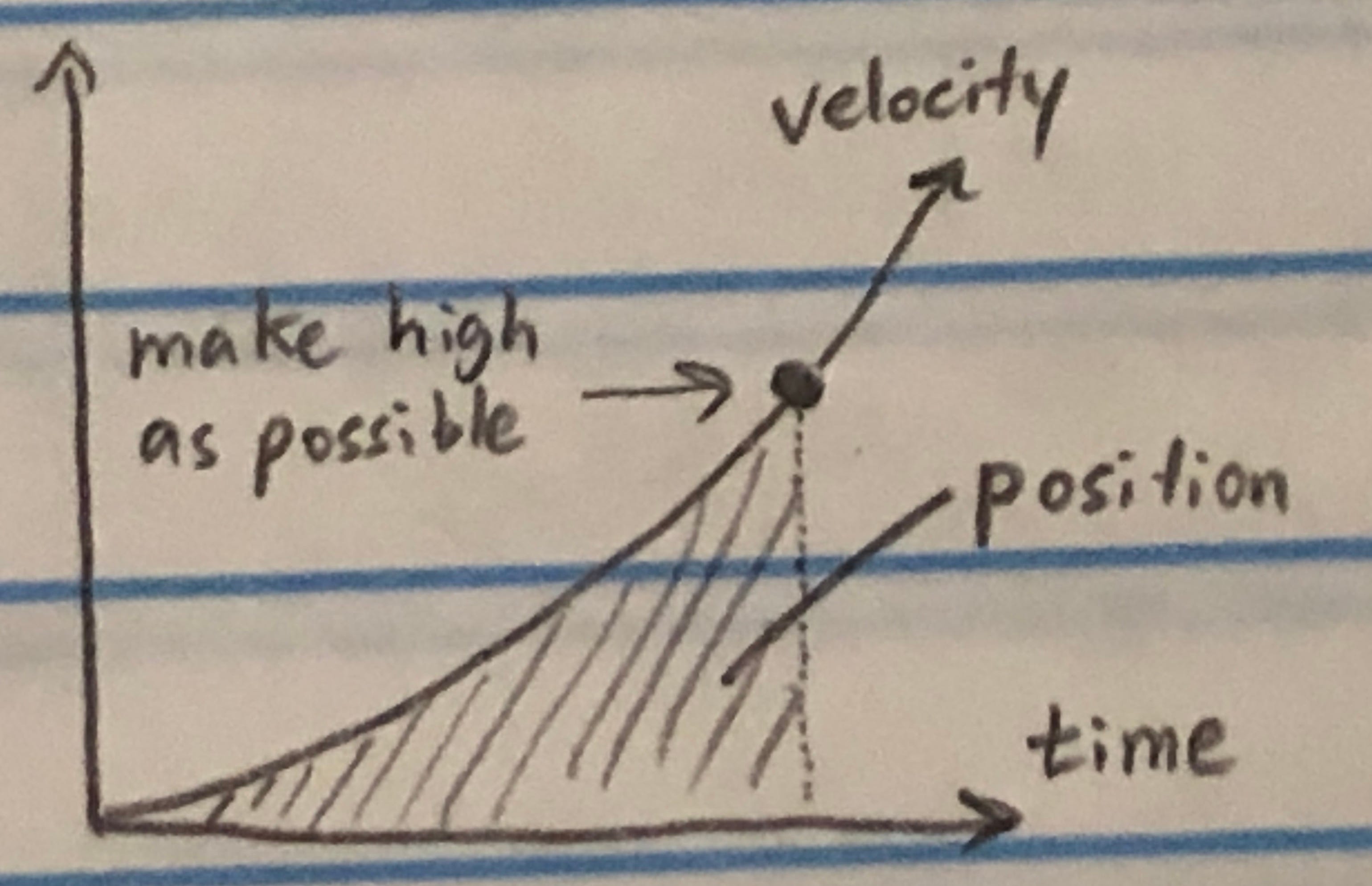
After the leg extends all the way, the jump is over and no more energy can be put into the system. To make the ending velocity as high as possible without “using up” too much position, the velocity plot should curve upwards to shrink the area underneath the curve. In the extreme case, the velocity stays flat until the very end, then it spikes up. This is accomplished when the leg is held still but power is still fed into the system, then all the stored energy is released at once.
A similar idea is applied in the Salto robot3. The system can be roughly represented by something like this, where there is also a transmission between the spring and the leg:

The second transmission isn’t a set of gears though, it has a variable mechanical advantage that changes as a function of the leg extension. Called series-elastic power modulation, the mechanical advantage transitions from low to high as the leg extends.
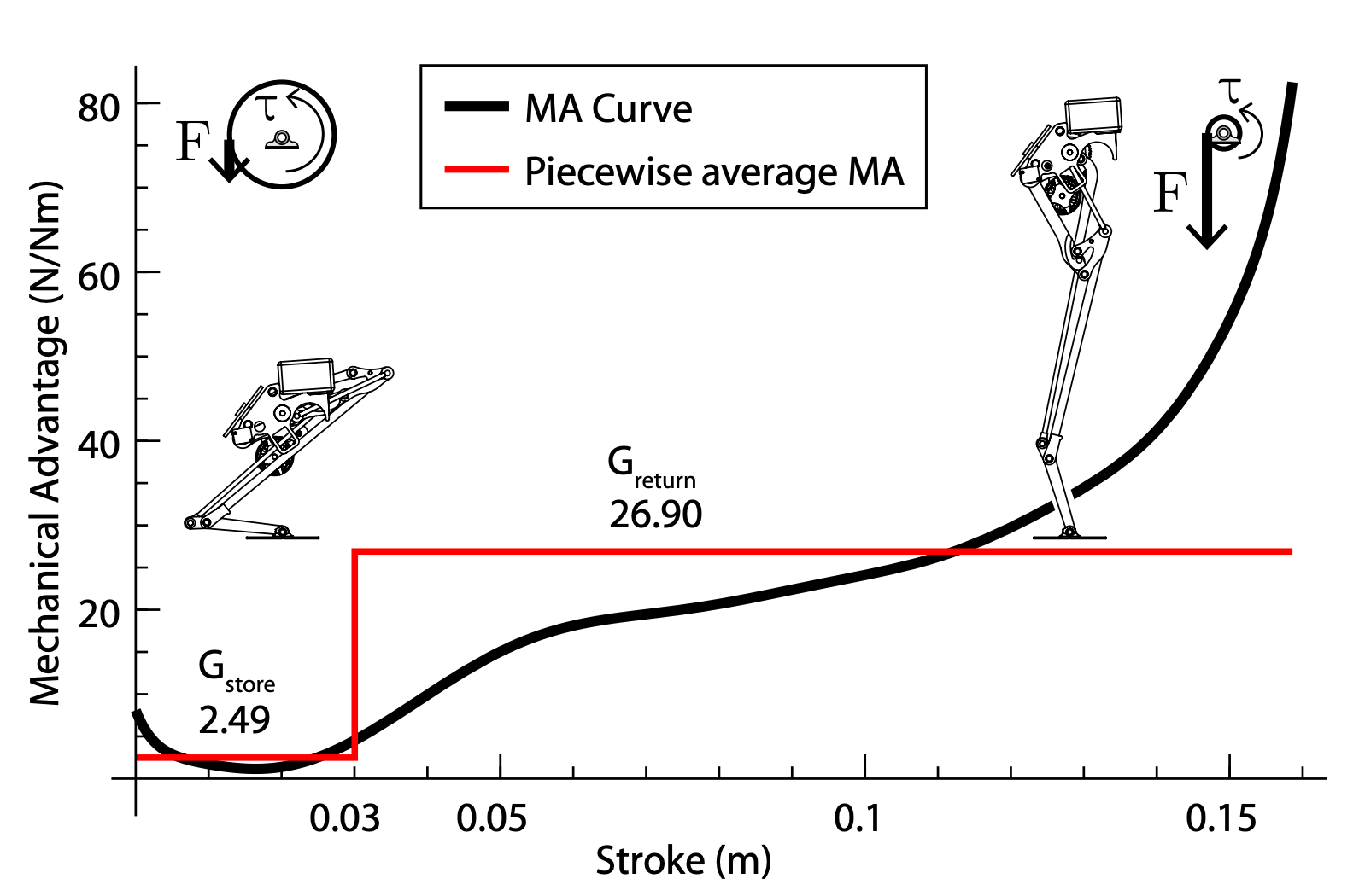
In the low mechanical advantage region at the beginning, the motor can wind up the spring without the leg moving very much, because it takes a lot of input force to achieve enough output force at the leg to accelerate it against gravity. At a certain point, there is enough spring force to move the leg into the high mechanical advantage region, where energy can be quickly released because the same spring force input results in a much higher leg force output.
The main idea is that the spring and transmission can be designed in a way where the motor spends more time applying power than if it were to directly accelerate the leg.
Physics model
If we create a generalized system that combines these concepts (varying mechanical advantage, series elasticity, storage & release periods) using a set of common parameters, then we can try to figure out when it is best to use each strategy by finding the optimal set of parameter values.
I will use the system below:

For simplicity, everything happens in a line (1D) and in a series chain. From left to right, the symbols represent:
Vertical line with hatched lines: the fixed point where the motor is attached
Piston looking thing: the part of the motor that applies force τa
Box ma: mass of the motor, with position xa
Hexagon T1: arbitrary transmission between motor and spring
Zigzag line: spring, where the positions of the endpoints are x1 and x2
Hexagon T2: arbitrary transmission between the spring and the load mass
Box mL: load mass to be accelerated
The jumping leg is slightly different because the motor is not fixed in place and the thing it pushes on is really the earth, but it should model most of the dynamics of the leg if we set ma to be the rotational inertia of the motor and mL to be the mass of the whole robot.
According to Justin Yim, one of the creators of Salto, the dynamics of the brushless motor are much faster than the whole jumping leg. To simplify the math, I’ll set ma to zero.
The variables I will eventually optimize for are the transmissions T1 and T2, plus the spring stiffness. T1 and T2 can change as the jump occurs, so we aren’t just finding the optimal set values of the transmission, but the profile of how T1 and T2 change over time.
Equations of motion
For constant T1 and T2, how the system moves can be described by a linear system of differential equations (from Lagrangian mechanics and linear motor model):

where x is a vector that contains the values of the motor position xa, load mass position xL, and the load mass velocity vL. The variables k, ωmax, and τmax represent the spring stiffness, maximum speed of the motor, and maximum torque of the motor. T1 and T2 are the transmission ratios: the ratio of speed out/speed in, analogous to gear ratio. This is the reciprocal of mechanical advantage (1/MA), and is used to make the expression slightly nicer.
Assuming constant T1 and T2 is useful because it allows us generate a closed-form solution to the differential equation for any initial condition (code here):
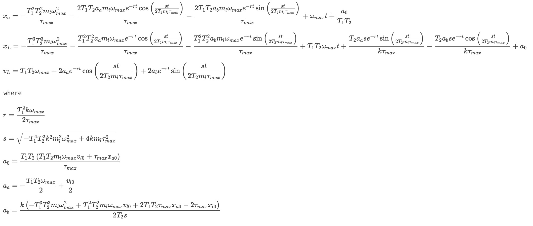
Now, we can write code to quickly and accurately solve for the state of the system at any time t. To account for varying T1 and T2, we can evaluate this solution in steps, using the final position from the previous step as the initial condition for the next.

Caveat: positions are calculated using x1 = T1xa and xL = T2x2. When T1 or T2 changes suddenly, the distance between x1 and x2 also changes suddenly, making it seem like the spring (whose length is defined by x2 – x1) is deforming for no reason. Because transmission ratio only deals with relative position, we can use xL = T2x2 + cL, where cL is a constant. In my implementation, when transferring the initial condition from one step to the next, I solve for the xL that keeps the spring compression continuous and therefore still physically accurate.
Computer thoughts
The algebra is a bit complicated, but it’s nice that a computer can do most of the work now that the problem is well defined. Given certain restrictions on the max motor speed, max motor torque, leg length, and time period, we want to find T1 and T2 to have the highest ending velocity.
Constant T
For constant T1 and T2, the map from transmission ratios to ending velocity looks like this:

Somewhere in the middle, there is a perfect balance of T1 and T2 that maximizes the power output of the motor, and a computer can quickly find this point:
I’m using the ipopt algorithm with CasADi to perform gradient-based optimization. Given an objective function, some constraints, and an initial input guess, it tries adjusting the function’s inputs in various directions until the objective function is maximized. The previous gif shows the algorithm converging to the same optimal point from randomized initial guesses.
Variable T and k
We want to find the best spring stiffness k by adding that as a parameter to optimize. Visualization gets harder when we also allow T1 and T2 to vary with time, because there are now 2*n+1 parameters to optimize, where n is the number of steps. More steps means more resolution at the cost of more compute time.
Here are the results from two similar runs, with constraints that the leg must lift off by 0.2 s, and the leg can extend at maximum 0.1 m:
The cool thing about profile optimization is that I gave no advice to the optimizer about what kind of strategy to use, it just finds one. Its strategy can be seen in the plot with the tradeoff between kinetic and potential energy. For most of the jump, the kinetic energy stays flat while potential energy increases linearly, meaning the motor is operating at a constant power and channelling all of it into the spring. At the last step, all the potential energy is converted into kinetic energy, creating a velocity spike. This can be accomplished by a T1 that continuously decreases and a T2 that stays high for most of the jump then suddenly drops low.
Transmission ratio T is the reciprocal of mechanical advantage, so this optimizer says mechanical advantage between the motor and spring should increase, and the mechanical advantage between the spring and the leg should be low all the way until the end. It seems that this optimizer found a strategy similar to Salto’s series-elastic power modulation described earlier: the leg does not move very much for the initial part of the jump so the spring can store more energy.

A difference is that the optimizer makes the transmission T1 before the spring a variable transmission. The mechanical advantage increases with time, meaning for the same force input there is an increasingly higher force output, but moving slower. This makes sense for the type of spring modeled here (Hookean spring), because as the spring gets more deformed, the force required to deform it further increases. To allow the motor to continue operating at its favorite speed/torque, the mechanical advantage should increase as more energy is stored into the spring. We can see that the motor velocity and power stays roughly constant in the first and last plot.
Predicting optimal T1
Actually, we can predict what the optimized T1 should be. If the leg does not move at all while the motor winds up the spring, setting the spring force equal to the motor force results in an inverse square root relationship between T1 and xa:

The T1 found by the optimizer does not completely match the case where the leg does not move (T2 → infinity), but it’s pretty close. Accounting for the movement caused by a finite T2 allows us to predict the optimized T1 almost perfectly.

Optimizing again and again
Energy storage/release with series-elastic power modulation happened to be the solution that the optimizer found for one set of physical constants and a particular random initial guess. Even in the constant transmission ratio case, it is obvious that changing the physical constants will affect the solution.
Are there other strategies that are not discovered due to the random guess chosen? What if a different overall strategy works better for other physical configurations of the problem?
“Random” guesses
With many optimization variables and such a complicated objective function, there are likely many local minima. The optimizer may think it found the best value, but it really is just on a peak that is higher than the surrounding area, while a taller peak exists out of reach. By running the optimizer many times starting from different places, the hope is that they will converge onto something that is very good overall.
However, uniform random sampling isn’t the most efficient way to explore the whole design space (consisting of permutations of T1, T2, k). Uniform random sampling has a good chance of reusing points that have appeared before, and optimizing from nearly the same place doesn’t give as much information. Latin Hypercube Sampling and Sobol sequences helps to sample points that are more equally distributed (reducing the discrepancy).

Here, I use Latin Hypercube Sampling because I want to cover as much of the design space as possible with not too many optimization runs (each optimization takes a few seconds). For the number of dimensions and samples, Sobol sequences take much longer to generate. Out of 60 optimizations, the top 15 are displayed here:

Seems like the various optimizations generally agree on the same strategy: decreasing T1 to wind up the spring with constant motor speed, then rapid change in T2 to release the energy.
Effect of spring stiffness
I sampled and optimized for 71 profiles for T1, T2, and spring stiffness k, shown below. To check the effect of spring stiffness, k was constrained during optimization to various regions (0–1000, 1000–2000, 2000–3000, etc) to find and compare the best values in each region.

For the parameters used, the optimum value for spring stiffness k is around 500 N/m, and restricting k to ranges that were strictly greater than 500 resulted in the optimizer choosing k to be the lowest number of the range. However, the difference in ending velocity is very small and a stiffness of 3000 N/m performed similarly (performance seems to drop off slowly after 3000 N/m). Below 300 N/m performance decreased dramatically, probably because it was not fast enough to propel the leg within one simulation time step and therefore wastes a time step of motor power.
This is good news for us building the physical robot, because we then have the flexibility to choose a spring stiffness using other considerations (manufacturing, force control bandwidth, effective stiffness at the foot) without affecting the jumping performance. Interestingly, many animals of different sizes that walk, trot, and hop have about the same relative stiffness per leg, and it can be shown that relative stiffness for a spring linear inverted pendulum hopping model is constant for dynamically similar motions4. Maybe we select a spring stiffness that matches those of animals.
Parameter sweep
What about different values for the mass of the leg, length of the leg, and time allotted? To get an insight on how these values affect the optimization, I repeated the previous optimizations for 5 values of mass (0.1–1 kg), 5 values of length (0.01–0.3 m), and 5 values of time (0.05–0.2 s) for a total of 125 different combinations.
In most cases, the leg does not move for most of the jump time and then suddenly snaps into motion at the last moment, which I’ll call the hold-release strategy. In the plots below, a hold-release strategy is identified by a continuously increasing orange line (potential energy) until the last step. Another strategy is accelerate the leg immediately, which I’ll call the direct-drive strategy. In the plots below, a direct-drive strategy is identified by a continuously increasing blue line (kinetic energy).
Increasing mass makes the direct-drive strategy more preferable and significantly reduces jump speed.

Increasing time allotted for the jump makes the hold-release strategy more preferable and significantly improves jump speed.

Increasing leg length makes the direct-drive strategy more preferable but does not usually improve jump speed:

I am guessing that the transition between the direct-drive and hold-release strategies happens at the point where applying the maximum motor power to the leg would make it extend to its limit before the allotted time. For direct-drive, the motor can apply power very efficiently for the period of time when the leg is within its extension limit. Any allotted time after that is wasted, because the leg can extend no further. On the other hand, hold-release allows motor power to be applied for an arbitrarily long period of time, but doesn’t always keep the motor operating at its best because it spins a bit too fast at the beginning and the end (and has spring damping losses, which is not modeled here).
The direct-drive strategy might not be effective for systems with lower mass, longer time, and shorter legs because they are likely to hit the extension limit.
One interesting result is that the hold-release strategy is present in the top 5 transmission profiles for each of the parameter combinations, though it might not be the best performing. However, when the hold-release strategy is preferable, it is the only strategy in the top 5. This may be due to the specific range of values I chose to explore, but it can also suggest that this strategy is more flexible to disturbances.
Takeaway
I find it very satisfying to use a computer to generate strategies from scratch, plus they make logical sense and can be seen in other impressive work like Minitaur and Salto. Overall, it seems like the hold-release strategy is the most promising for our squirrel leg:
Use some sort of latch to hold the leg in place.
Gradually increase the mechanical advantage to wind up a spring at a constant motor speed
Suddenly release the leg to convert elastic energy to kinetic energy.
The explorations above show that this strategy is (probably) optimal in a wide range of scenarios we are likely to work with, and the only precision we need is to match T1 with the spring stiffness and motor characteristics.
Limitations
I learned a lot in the process of modeling the system, solving its differential equation, running simulations, and optimizing various variables. However, the results can’t be fully trusted because:
There should be a constant backwards gravity force on the leg, which would affect how fast it is able to accelerate. It is not modeled because I did not want to deal with the case when the leg force cannot overcome gravity and the body is instead supported by contact with an end stop. In one example configuration, the work done by gravity for leg extension is roughly 7% of the total jump energy.
Possible next step: Numerically simulate the system with the same parameters but with gravity and check model similarity. Hopefully, the jump is a consistent amount slower but the optimal strategies stay the same.
Most results that involve repeated optimizations used only 20 steps for computation speed. Although the closed form solution should be precise, the transmission ratio profiles T1 and T2 can only change every step. T1 is likely to be implemented with a linkage and would be continuous in reality. The precise moment T2 suddenly decreases in transmission ratio is important for the spring hold-release strategy, and only having a discrete selection of times limits the optimization. The last step is usually reserved for the spring release, but the step size may be shorter or longer than truly optimal.
Possible next step: use the theoretical T1(x) profile and simulate how it does using numerical integration, then compare with current results.
Possible next step: introduce another optimization variable that determines the times when the steps occur. This should find the best time to release the spring in the hold-release strategy.