Extra: Linkage optimization

Finding straight line paths with CMA-ES

This is an extra post about the technical process for optimizing the geometry of the 4-bar linkage used in the test stand boom arm. 

Instead of following an arc if the boom arm were simply on a rotational joint, we want to constrain the leg to a purely vertical motion so there would be more uniform forces on the leg that are a closer representation of a full squirrel jump. 

We can choose the exact dimensions of the linkage lengths to constrain the leg to the path we want. If chosen manually by intuition, the system will likely still work, but as practice for future iterations of the squirrel leg, we performed linkage optimization with CMA-ES to maximize the allowed jump height.

The structure of the linkage looks like this:

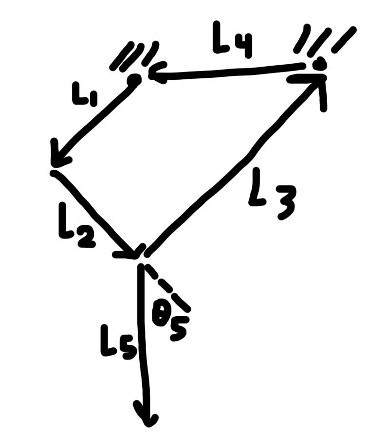
Link L4 is completely fixed and L5 is rigidly attached to L2 at some angle, so there is one degree of freedom. This structure comes from the Chebyshev lambda linkage, which for certain link proportions the end effector traces almost a straight line for a considerable portion of its path. Other straight line mechanisms exist, but this one is simple and keeps the end effector far away, so we can have mainly short links close to the attachment point to keep the inertia low (as experienced by the leg). 

The goal is to create a 4-bar linkage whose end effector moves vertically in a straight line path. Here’s the overview of the process:

• Start with the Chebyshev lambda linkage. Fix the length of L5 to 500mm (length of many off-the-shelf carbon fiber rods) and try various values for L1, L2, L3, L4, and θ5.

• Iterate through 50 evenly spaced angles for L1. Solve a loop closure equation to get the position of the end effector (end of L5) at each angle to build a path.

• Some parts of the path are not usable because the 4-bar reaches something like a kinematic singularity. Restrict the path to a continuous section that is well-behaved using the transmission ratio.

• Apply the Douglas-Peucker algorithm to find the longest straight section of the path

• Repeat last 4 steps repeatedly, using a CMA-ES library that tries to maximize the length of the longest straight section using an evolutionary strategy.

---

Loop closure

We find the path of the end effector by solving a vector loop closure equation for L1, L2, L3, and L4. With the vector directions specified in the sketch above,  

\(\overline{L1}+\overline{L2}+\overline{L3}+\overline{L4}=0\)

Written as scalar equations, one equation each for x and y coordinate:

\(\begin{bmatrix} L_1 \cdot \sin(\theta_1) + L_2 \cdot \sin(\theta_2) + L_3 \cdot \sin(\theta_3)=0 \\ L_1 \cdot \cos(\theta_1) + L_2 \cdot \cos(\theta_2) + L_3 \cdot \cos(\theta_3) - L_4=0 \\ \end{bmatrix}\)

The lengths of the links and θ₁ will be constants, and solving for θ₂ and θ₃ will give us the angles and therefore the position of each joint in the linkage. Unfortunately, we couldn’t get the closed form solution for the angles. 

This should be ready to plug into scipy’s root(method=’hybr’) solver for nonlinear systems of equations, but for faster computation, we can solve for the sine and cosine values instead of the θ angles themselves:

\(\begin{bmatrix} L_1 \cdot s_1 + L_2 \cdot s_2 + L_3 \cdot s_3=0 \\ L_1 \cdot c_1 + L_2 \cdot c_2 + L_3 \cdot c_3 - L_4=0 \\ s_1^2+c_1^2-1=0 \\ s_2^2+c_2^2-1=0 \\ \end{bmatrix}\)

There are now 4 variables to simultaneously solve for, but there are no longer trigonometric function evaluations, which happened to be slightly faster.

To speed up the solver more, we provide the solver with the jacobian:

\(\begin{bmatrix}     L_2 & 0 & L_3 & 0 \\     0 & L_2 & 0 & L_3 \\     2 s_2 & 2 c_2 & 0 & 0 \\     0 & 0 & 2 s_3 & 2 c_3 \end{bmatrix}\)

Each solve (contributing to a single point on the linkage path) took around 31μs to complete. Newton-Raphson’s method to calculate the inverse jacobian was also tried, but turned out to be slower. 

After knowing the angle components of L2 and L3, we can quickly find the position of the end effector by adding the vectors:

\(p_5 = L_1 \cdot \begin{bmatrix} \cos(\theta_1) \\ \sin(\theta_1) \end{bmatrix} + L_2 \cdot \begin{bmatrix} \cos(\theta_2) \\ \sin(\theta_2) \end{bmatrix} + L_5 \cdot \begin{bmatrix} \cos(\theta_2) \cdot \cos(\theta_5) - \sin(\theta_2) \cdot \sin(\theta_5) \\ \sin(\theta_2) \cdot \cos(\theta_5) + \cos(\theta_2) \cdot \sin(\theta_5) \end{bmatrix}\)

---

Transmission ratio:

At some points during the path, the 4-bar reaches something like a kinematic singularity and the end-effector moves much faster than usual for the same variation in the L1 angle. Also, these are points where the linkage can diverge into two possible configurations. To avoid these points, we impose an upper limit on the transmission ratio between the L1 angle and the angle that the end effector has with the origin (using an approximation that the end effector moves in a 500mm radius arc). We found that using a threshold of 0.7 works well in finding the straighter parts of the path. In other words, we only use the longest continuous section of the path where a 1º/sec rotation in L1 will move the end effector no faster than 0.7º/sec. 

---

Straightness metric

We can measure the “straightness” of a path using the Douglas-Peucker algorithm, which is used to efficiently simplify a series of line segments based on how far each point deviates from a straight line. More specifically, this algorithm recursively approximates a complex path using progressively more line segments until every point on the true path is within some perpendicular distance to the approximated path. The effect is that running this algorithm allows us to find the longest section of the end effector path within some straightness threshold. We specified this threshold to be 1mm, because variations less than this from a straight line is likely unnoticeable given the flexibility and backlash in the system.

---

Optimization with CMA-ES

CMA-ES is an evolutionary strategy algorithm to iteratively find better combinations of variables that have higher fitness value than the last. It is vulnerable to local minima and its solution depends heavily on the initial guess, but it works here to explore the design space of link lengths and angle to use that maximize the straightest linear section of the linkage path. We are using this python library’s implementation, which which simply takes the variables you have control over and a callable fitness function to maximize.

• Variables: 

  • Lengths of L1, L2, L3, L4

  • Angle θ₅, which fixes the angle between L2 and L5

• Fitness function: Length of the longest segment after running Douglas-Peucker on the longest continuous segment under a transmission ratio

  • Constraints

    • L1, L2, L3, and L4 must each be shorter than 50mm. This is to keep everything other than the boom arm close to the fixed attachment point and low inertia.

    • built into the fitness function by immediately returning zero fitness when a constraint is violated.

• Parameters:

  • Straightness threshold (epsilon): 1mm

  • Transmission ratio cutoff: 0.7

    ---

    

    Yay, it’s pretty much a straight line! This linear portion is about 250mm long.

Code here